Note
Click here to download the full example code
SPGL1 Tutorial
In this tutorial we will explore the different solvers in the spgl1
package and apply them to different toy examples.
import numpy as np
import matplotlib.pyplot as plt

from scipy.sparse.linalg import LinearOperator
from scipy.sparse import spdiags
import spgl1

# Initialize random number generators
np.random.seed(43273289)
Create random m-by-n encoding matrix and sparse vector
Solve the underdetermined LASSO problem for \(||\mathbf{x}||_1 <= \pi\):
b = A.dot(x0)
tau = np.pi
x, resid, grad, info = spgl1.spg_lasso(A, b, tau, verbosity=1)

print('%s%s%s' % ('-'*35, ' Solution ', '-'*35))
print('nonzeros(x) = %i,   ||x||_1 = %12.6e,   ||x||_1 - pi = %13.6e' %
      (np.sum(np.abs(x) > 1e-5), np.linalg.norm(x, 1),
       np.linalg.norm(x, 1)-np.pi))
print('%s' % ('-'*80))
Out:
================================================================================
SPGL1
================================================================================
No. rows              :       50
No. columns           :      128

Initial tau           : 3.14e+00
Two-norm of b         : 3.40e+00

Optimality tol        : 1.00e-04
Target one-norm of x  : 3.14e+00

Basis pursuit tol     : 1.00e-06
Maximum iterations    :      500


EXIT -- Optimal solution found

Products with A     :       8        Total time   (secs) :     0.0
Products with A^H   :       8        Project time (secs) :     0.0
Newton iterations   :       0        Mat-vec time (secs) :     0.0
Line search its     :       0        Subspace iterations :       0
----------------------------------- Solution -----------------------------------
nonzeros(x) = 7,   ||x||_1 = 3.141593e+00,   ||x||_1 - pi =  0.000000e+00
--------------------------------------------------------------------------------
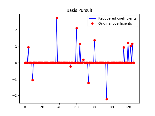
Solve the basis pursuit (BP) problem:
\[min. ||\mathbf{x}||_1 \quad subject \quad to \quad \mathbf{Ax} = \mathbf{b}\]
b = A.dot(x0)
x, resid, grad, info = spgl1.spg_bp(A, b, verbosity=2)
plt.figure()
plt.plot(x, 'b')
plt.plot(x0, 'ro')
plt.legend(('Recovered coefficients', 'Original coefficients'))
plt.title('Basis Pursuit')
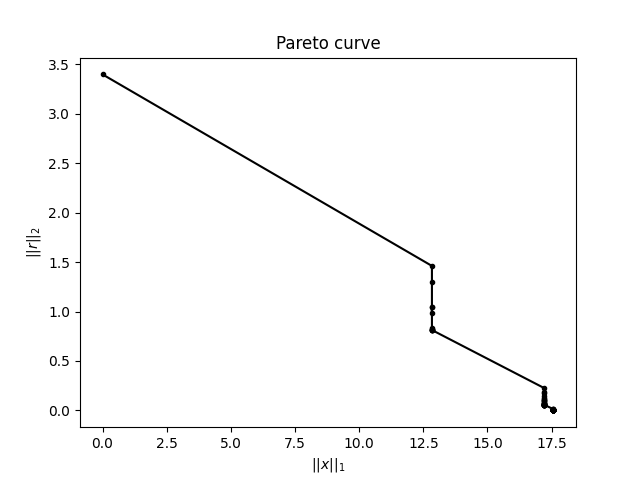
plt.figure()
plt.plot(info['xnorm1'], info['rnorm2'], '.-k')
plt.xlabel(r'$||x||_1$')
plt.ylabel(r'$||r||_2$')
plt.title('Pareto curve')
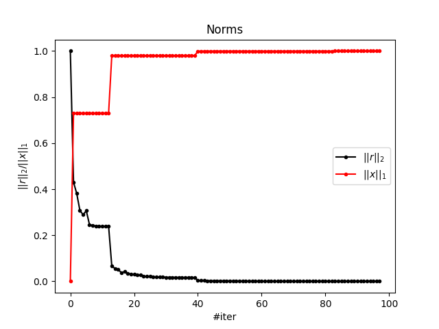
plt.figure()
plt.plot(np.arange(info['niters']), info['rnorm2']/max(info['rnorm2']),
'.-k', label=r'$||r||_2$')
plt.plot(np.arange(info['niters']), info['xnorm1']/max(info['xnorm1']),
'.-r', label=r'$||x||_1$')
plt.xlabel(r'#iter')
plt.ylabel(r'$||r||_2/||x||_1$')
plt.title('Norms')
plt.legend()
Out:
================================================================================
SPGL1
================================================================================
No. rows              :       50
No. columns           :      128

Initial tau           : 0.00e+00
Two-norm of b         : 3.40e+00

Optimality tol        : 1.00e-04
Target objective      : 0.00e+00

Basis pursuit tol     : 1.00e-06
Maximum iterations    :      500

iterr      Objective   Relative Gap  Rel Error      gnorm   stepg   nnz_x   nnz_g     tau

    0  3.3978494e+00  0.0000000e+00   1.00e+00  8.995e-01     0.0       0       0  1.2834830e+01
    1  1.4610032e+00  1.6532743e+00   1.00e+00  3.459e-01    -0.6      67       1
    2  1.2957367e+00  1.4480527e+00   1.00e+00  3.057e-01     0.0      53       1
    3  1.0445582e+00  1.0186987e+00   1.00e+00  2.394e-01     0.0      33       1
    4  9.8320803e-01  1.9671347e+00   9.83e-01  3.006e-01     0.0      17       1
    5  1.0408537e+00  2.7237524e+00   1.00e+00  3.273e-01     0.0      15       1
    6  8.3766484e-01  4.4627639e-01   8.38e-01  1.829e-01     0.0      20       1
    7  8.2370803e-01  2.1784189e-01   8.24e-01  1.661e-01     0.0      16       1
    8  8.1471442e-01  1.0576174e-01   8.15e-01  1.582e-01     0.0      15       1
    9  8.1352564e-01  1.2833205e-01   8.14e-01  1.618e-01     0.0      12       2
   10  8.1346284e-01  1.2136051e-01   8.13e-01  1.595e-01     0.0      12       3
   12  8.1283336e-01  1.6431186e-03   8.13e-01  1.509e-01     0.0      12      12  1.7214207e+01
   20  1.0262800e-01  3.7124664e-02   1.03e-01  1.684e-02     0.0      55       5
   30  5.8775070e-02  2.1151854e-02   5.88e-02  9.905e-03     0.0      26       5
   39  5.6081993e-02  3.4487799e-03   5.61e-02  9.059e-03     0.0      16      16  1.7561410e+01
   40  1.3497461e-02  2.3368157e-02   1.35e-02  2.563e-03     0.0      61      17
   50  6.5248570e-03  2.5729401e-02   6.52e-03  2.012e-03    -0.6      44       8
   60  3.6779037e-03  8.0294188e-03   3.68e-03  8.458e-04    -0.9      30      30
   70  1.7198692e-03  6.8520394e-04   1.72e-03  2.801e-04     0.0      17      17
   80  1.3668596e-03  8.5588974e-05   1.37e-03  2.204e-04     0.0      14      14
   82  1.3666459e-03  1.8193226e-05   1.37e-03  2.163e-04     0.0      14      14  1.7570044e+01
   90  1.3860943e-04  4.2028246e-05   1.39e-04  2.222e-05     0.0      14      14
   98  8.6425580e-05  5.4782377e-05   8.64e-05  1.545e-05     0.0      14      14

EXIT -- Found a root

Products with A     :     131        Total time   (secs) :     0.0
Products with A^H   :      99        Project time (secs) :     0.0
Newton iterations   :       4        Mat-vec time (secs) :     0.0
Line search its     :      32        Subspace iterations :       0

<matplotlib.legend.Legend object at 0x7fdfcc084e48>
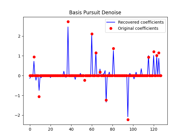
Solve the basis pursuit denoise (BPDN) problem:
b = A.dot(x0) + np.random.randn(m) * 0.075
sigma = 0.10  # Desired ||Ax - b||_2
x, resid, grad, info = spgl1.spg_bpdn(A, b, sigma, iter_lim=100, verbosity=2)

plt.figure()
plt.plot(x, 'b')
plt.plot(x0, 'ro')
plt.legend(('Recovered coefficients', 'Original coefficients'))
plt.title('Basis Pursuit Denoise')
Out:
================================================================================
SPGL1
================================================================================
No. rows              :       50
No. columns           :      128

Initial tau           : 0.00e+00
Two-norm of b         : 3.49e+00

Optimality tol        : 1.00e-04
Target objective      : 1.00e-01

Basis pursuit tol     : 1.00e-06
Maximum iterations    :      100

iterr      Objective   Relative Gap  Rel Error      gnorm   stepg   nnz_x   nnz_g     tau

    0  3.4876525e+00  0.0000000e+00   9.71e-01  8.998e-01     0.0       0       0  1.3130733e+01
    1  1.5278506e+00  1.5445083e+00   9.35e-01  3.512e-01    -0.6      70       1
    2  1.3785367e+00  1.3210423e+00   9.27e-01  3.004e-01     0.0      48       1
    3  1.1435885e+00  1.0754951e+00   9.13e-01  2.436e-01     0.0      36       1
    4  1.0650070e+00  1.8808347e+00   9.06e-01  3.058e-01     0.0      24       1
    5  1.1055544e+00  1.9676460e+00   9.10e-01  2.609e-01     0.0      14       1
    6  9.7104698e-01  5.0757852e-01   8.71e-01  1.910e-01     0.0      21       1
    7  9.5573059e-01  2.5393233e-01   8.56e-01  1.677e-01     0.0      20       1
    8  9.5003110e-01  1.6053048e-01   8.50e-01  1.613e-01     0.0      19       1
    9  9.4642238e-01  6.3958437e-02   8.46e-01  1.545e-01     0.0      16       1
   10  9.4667260e-01  1.0342969e-01   8.47e-01  1.576e-01     0.0      15       1
   12  9.4626463e-01  5.7319569e-03   8.46e-01  1.499e-01     0.0      15      15  1.8472152e+01
   20  1.9419435e-01  4.1553930e-02   9.42e-02  2.642e-02     0.0      46       4  1.9164449e+01
   30  1.0621175e-01  1.0890316e-02   6.21e-03  1.305e-02     0.0      48      38
   40  1.0446001e-01  4.9732393e-03   4.46e-03  1.269e-02     0.0      47      47  1.9201152e+01
   41  1.0004744e-01  1.2472217e-02   4.74e-05  1.237e-02     0.0      47      46

EXIT -- Found a root

Products with A     :      53        Total time   (secs) :     0.0
Products with A^H   :      42        Project time (secs) :     0.0
Newton iterations   :       4        Mat-vec time (secs) :     0.0
Line search its     :      11        Subspace iterations :       0

Text(0.5, 1.0, 'Basis Pursuit Denoise')
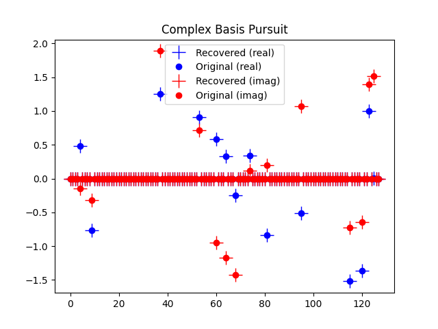
Solve the basis pursuit (BP) problem in complex variables:
\[min. ||\mathbf{z}||_1 \quad subject \quad to \quad \mathbf{Az} = \mathbf{b}\]
class partialFourier(LinearOperator):
    def __init__(self, idx, n):
        self.idx = idx
        self.n = n
        self.shape = (len(idx), n)
        self.dtype = np.complex128
    def _matvec(self, x):
        # % y = P(idx) * FFT(x)
        z = np.fft.fft(x) / np.sqrt(n)
        return z[idx]
    def _rmatvec(self, x):
        z = np.zeros(n, dtype=complex)
        z[idx] = x
        return np.fft.ifft(z) * np.sqrt(n)

# Create partial Fourier operator with rows idx
idx = np.random.permutation(n)
idx = idx[0:m]
opA = partialFourier(idx, n)

# Create sparse coefficients and b = A * z0
z0 = np.zeros(n, dtype=complex)
z0[p] = np.random.randn(k) + 1j * np.random.randn(k)
b = opA.matvec(z0)

# Solve problem
z, resid, grad, info = spgl1.spg_bp(opA, b, verbosity=2)

plt.figure()
plt.plot(z.real, 'b+', markersize=15.0)
plt.plot(z0.real, 'bo')
plt.plot(z.imag, 'r+', markersize=15.0)
plt.plot(z0.imag, 'ro')
plt.legend(('Recovered (real)', 'Original (real)',
            'Recovered (imag)', 'Original (imag)'))
plt.title('Complex Basis Pursuit')
Out:
================================================================================
SPGL1
================================================================================
No. rows              :       50
No. columns           :      128

Initial tau           : 0.00e+00
Two-norm of b         : 3.23e+00

Optimality tol        : 1.00e-04
Target objective      : 0.00e+00

Basis pursuit tol     : 1.00e-06
Maximum iterations    :      500

iterr      Objective   Relative Gap  Rel Error      gnorm   stepg   nnz_x   nnz_g     tau

    0  3.2278608e+00  0.0000000e+00   1.00e+00  9.900e-01     0.0       0       0  1.0524266e+01
    1  1.7448418e+00  1.9165918e+00   1.00e+00  5.168e-01    -0.6      95       0
    2  1.4600574e+00  1.5883031e+00   1.00e+00  3.875e-01     0.0      57       0
    3  1.1700012e+00  7.2057823e-01   1.00e+00  2.294e-01     0.0      21       0
    4  1.1387081e+00  6.0492162e-01   1.00e+00  2.591e-01     0.0      14       0
    5  1.1192644e+00  6.3143375e-01   1.00e+00  2.339e-01     0.0      13       0
    6  1.1110267e+00  2.5990247e-02   1.00e+00  1.887e-01     0.0      14       1
    7  1.1109277e+00  1.8665102e-02   1.00e+00  1.882e-01     0.0      14       1
    8  1.1109130e+00  9.8075649e-03   1.00e+00  1.876e-01     0.0      14       1  1.7103189e+01
    9  4.0897300e-01  2.0290430e+00   4.09e-01  1.096e-01     0.0      33       0
   10  2.4260476e-01  3.0388666e-01   2.43e-01  5.139e-02     0.0      84       0
   20  7.3650715e-02  1.5598521e-01   7.37e-02  1.898e-02    -0.6      36       0
   30  3.9788017e-02  1.6542009e-03   3.98e-02  6.363e-03     0.0      15       6
   32  3.9782650e-02  1.1422412e-03   3.98e-02  6.356e-03     0.0      14       6  1.7352196e+01
   40  5.2988820e-03  2.3780254e-03   5.30e-03  8.349e-04     0.0      45      37
   50  1.0390591e-03  8.2222429e-04   1.04e-03  1.846e-04     0.0      14      14
   60  4.3109396e-04  2.4523963e-04   4.31e-04  8.092e-05     0.0      14      14
   65  4.2277734e-04  2.9843344e-06   4.23e-04  6.689e-05     0.0      14      14  1.7354868e+01
   68  6.8724121e-05  5.4983919e-05   6.87e-05  1.067e-05     0.0      14      14

EXIT -- Found a root

Products with A     :      85        Total time   (secs) :     0.0
Products with A^H   :      69        Project time (secs) :     0.0
Newton iterations   :       4        Mat-vec time (secs) :     0.0
Line search its     :      16        Subspace iterations :       0

Text(0.5, 1.0, 'Complex Basis Pursuit')
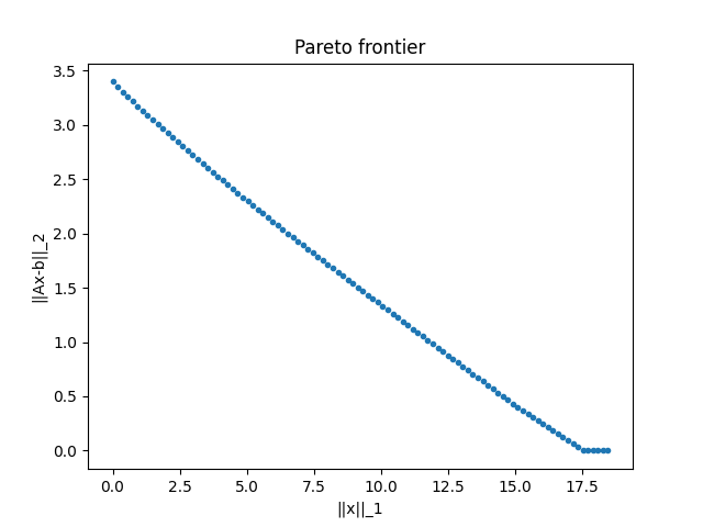
We can also sample the Pareto frontier at 100 points:
\[\phi(\tau) = min. ||\mathbf{Ax}-\mathbf{b}||_2 \quad subject \quad to \quad ||\mathbf{x}|| <= \tau\]
b = A.dot(x0)
x = np.zeros(n)
tau = np.linspace(0, 1.05 * np.linalg.norm(x0, 1), 100)
tau[0] = 1e-10
phi = np.zeros(tau.size)

for i in range(tau.size):
    x, r, grad, info = spgl1.spgl1(A, b, tau[i], 0, x, iter_lim=1000)
    phi[i] = np.linalg.norm(r)

plt.figure()
plt.plot(tau, phi, '.')
plt.title('Pareto frontier')
plt.xlabel('||x||_1')
plt.ylabel('||Ax-b||_2')
Out:
Text(42.722222222222214, 0.5, '||Ax-b||_2')
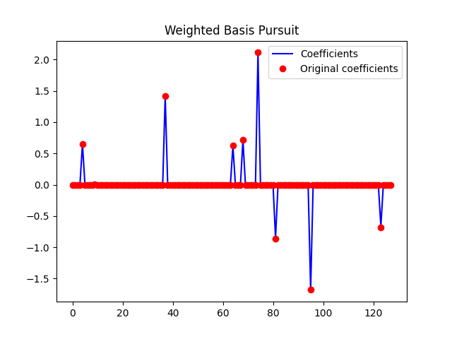
We now solve the weighted basis pursuit (BP) problem:
\[min. ||\mathbf{y}||_1 \quad subject \quad to \quad \mathbf{AW}^{-1}\mathbf{y} = \mathbf{b}\]
and
\[min. ||\mathbf{Wx}||_1 \quad subject \quad to \quad \mathbf{Ax} = \mathbf{b}\]
followed by setting :math`mathbf{y} = mathbf{Wx}`.
# Sparsify vector x0 a bit more to get exact recovery
k = 9
x0 = np.zeros(n)
x0[p[0:k]] = np.random.randn(k)

# Set up weights w and vector b
w = np.random.rand(n) + 0.1 # Weights
b = A.dot(x0 / w)  # Signal

# Solve problem
x, resid, grad, info = spgl1.spg_bp(A, b, iter_lim=1000, weights=w)

# Reconstructed solution, with weighting
x1 = x * w

plt.figure()
plt.plot(x1, 'b')
plt.plot(x0, 'ro')
plt.legend(('Coefficients', 'Original coefficients'))
plt.title('Weighted Basis Pursuit')
k = 9
x0 = np.zeros(n)
x0[p[0:k]] = np.random.randn(k)
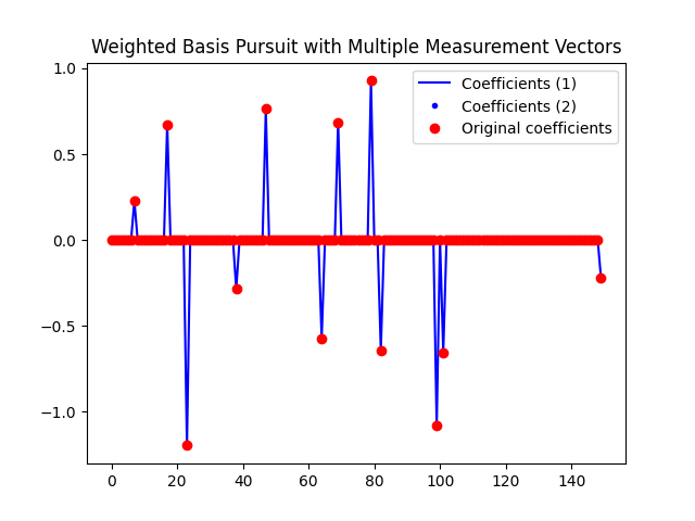
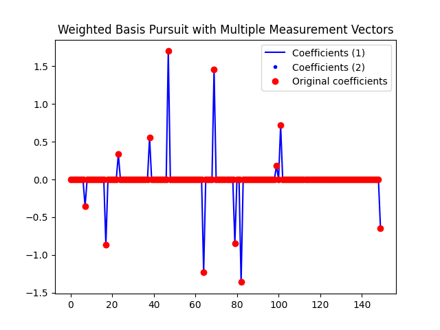
Finally we solve the multiple measurement vector (MMV) problem
\[min. | | \mathbf{Y} | |_{1, 2} \quad subject \quad to \quad \mathbf{AW}^{-1} \mathbf{Y} = \mathbf{B}\]
and the weighted MMV problem(weights on the rows of X):
\[min. | | \mathbf{WX} | |_{1, 2} \quad subject \quad to \quad \mathbf{AX} = \mathbf{B}\]
followed by setting \(\mathbf{Y} = \mathbf{WX}\).
# Create problem
m = 100
n = 150
k = 12
l = 6
A = np.random.randn(m, n)
p = np.random.permutation(n)[:k]
X0 = np.zeros((n, l))
X0[p, :] = np.random.randn(k, l)

weights = 3 * np.random.rand(n) + 0.1
W = 1/weights * np.eye(n)
B = A.dot(W).dot(X0)

# Solve unweighted version
x_uw, _, _, _ = spgl1.spg_mmv(A.dot(W), B, 0, verbosity=1)

# Solve weighted version
x_w, _, _, _ = spgl1.spg_mmv(A, B, 0, weights=weights, verbosity=2)
x_w = spdiags(weights, 0, n, n).dot(x_w)

# Plot results
plt.figure()
plt.plot(x_uw[:, 0], 'b-', label='Coefficients (1)')
plt.plot(x_w[:, 0], 'b.', label='Coefficients (2)')
plt.plot(X0[:, 0], 'ro', label='Original coefficients')
plt.legend()
plt.title('Weighted Basis Pursuit with Multiple Measurement Vectors')

plt.figure()
plt.plot(x_uw[:, 1], 'b-', label='Coefficients (1)')
plt.plot(x_w[:, 1], 'b.', label='Coefficients (2)')
plt.plot(X0[:, 1], 'ro', label='Original coefficients')
plt.legend()
plt.title('Weighted Basis Pursuit with Multiple Measurement Vectors')
Out:
================================================================================
SPGL1
================================================================================
No. rows              :      600
No. columns           :      900

Initial tau           : 0.00e+00
Two-norm of b         : 9.86e+01

Optimality tol        : 1.00e-04
Target objective      : 0.00e+00

Basis pursuit tol     : 1.00e-06
Maximum iterations    :     6000

/home/docs/checkouts/readthedocs.org/user_builds/spgl1/checkouts/latest/spgl1/spgl1.py:345: RuntimeWarning: invalid value encountered in true_divide
  xc = xc / xa

EXIT -- Found a BP solution

Products with A     :    4448        Total time   (secs) :     2.6
Products with A^H   :    2419        Project time (secs) :     1.8
Newton iterations   :      14        Mat-vec time (secs) :     0.2
Line search its     :    2029        Subspace iterations :       0

================================================================================
SPGL1
================================================================================
No. rows              :      600
No. columns           :      900

Initial tau           : 0.00e+00
Two-norm of b         : 9.86e+01

Optimality tol        : 1.00e-04
Target objective      : 0.00e+00

Basis pursuit tol     : 1.00e-06
Maximum iterations    :     6000

iterr      Objective   Relative Gap  Rel Error      gnorm   stepg   nnz_x   nnz_g     tau

    0  9.8602912e+01  0.0000000e+00   1.00e+00  1.017e+03     0.0       0       0  9.5554864e+00
    1  6.9417410e+01  1.9595302e+00   1.00e+00  6.916e+02    -0.6     419       0
    2  5.1761792e+01  1.3643668e+00   1.00e+00  4.022e+02     0.0     212       0
    3  4.4719199e+01  3.3088079e-01   1.00e+00  2.211e+02     0.0      96       0
    4  4.4235054e+01  3.9317252e-01   1.00e+00  2.183e+02     0.0      89       0
    5  4.4209620e+01  1.9011325e-01   1.00e+00  1.934e+02     0.0      88       0
    6  4.4195524e+01  3.7232090e-03   1.00e+00  1.767e+02     0.0      95       0
    7  4.4195175e+01  2.1356103e-03   1.00e+00  1.764e+02     0.0      95       0  2.0630352e+01
    8  2.1170991e+01  7.4323046e+00   1.00e+00  1.091e+02     0.0     334       0
    9  1.7331061e+01  2.2758703e+00   1.00e+00  5.633e+01     0.0     337       0
   10  1.5859590e+01  3.6326634e+00   1.00e+00  5.650e+01     0.0     293       0
   18  1.4217254e+01  4.3066544e-01   1.00e+00  3.173e+01     0.0     170       8  2.7000370e+01
   20  5.5823227e+00  1.3015844e+01   1.00e+00  1.551e+01     0.0     646       0
   30  2.4925735e+00  7.7271486e+00   1.00e+00  5.108e+00     0.0     196       4
   34  2.4883824e+00  7.4225525e-01   1.00e+00  4.266e+00     0.0     188      11  2.8451690e+01
   40  4.1105039e-01  5.9696329e+01   4.11e-01  2.529e+00     0.0     316       0
   50  1.0902142e-01  1.6349931e+00   1.09e-01  1.801e-01     0.0     137       4
   60  4.9748935e-02  1.8398584e+00   4.97e-02  1.471e-01     0.0      72       2
   63  4.9435528e-02  3.6531447e-02   4.94e-02  8.404e-02     0.0      72      12  2.8480769e+01
   70  1.1780283e-02  5.0958811e+00   1.18e-02  1.780e-01     0.0      72       0
   80  1.5540978e-03  4.8472422e-02   1.55e-03  3.408e-03     0.0      72       4
   90  6.7461437e-04  7.6278843e-03   6.75e-04  1.402e-03     0.0      72      34
   95  6.7316524e-04  1.4549718e-03   6.73e-04  1.180e-03     0.0      72      57  2.8481154e+01
  100  1.8442074e-04  9.0788110e-03   1.84e-04  5.075e-04     0.0      72      72
  103  9.4798950e-05  6.5696437e-03   9.48e-05  3.365e-04     0.0      72      72

EXIT -- Found a BP solution

Products with A     :     114        Total time   (secs) :     0.1
Products with A^H   :     104        Project time (secs) :     0.0
Newton iterations   :       6        Mat-vec time (secs) :     0.0
Line search its     :      10        Subspace iterations :       0

Text(0.5, 1.0, 'Weighted Basis Pursuit with Multiple Measurement Vectors')
Total running time of the script: ( 0 minutes 4.441 seconds)